session 11 (Exception Handling and Event Handling)

Exception Handling dan Event Handling

Exception

Dalam melakukan pemrograman pasti pernah terjadi kesalahan, hal tersebut secara otomatis akan dilemparkan dalam bentuk objek yang disebut sebagai exception. Secara lebih rinci, exception merupakan suatu event yang terjadi selama eksekusi program dan mengacaukan aliran normal instruksi program. Dalam menangani sebuah exception, Java menggunakan mekanisme penanganan exception terstruktur.

Contoh kasus yang sering dialami yaitu sebuah program apabila mengalami kesalahan akan menghasilkan suatu runtime errors seperti gagal membuka file. Ketika runtime error terjadi, maka aplikasi akan membuat suatu exception.

Exception juga memiliki berbagai macam operasi yang dapat terbagi menjadi 3 bagian besar yaitu

  1. Claiming an exception: ketika error terjadi di suatu method, maka method akan membuat objek yang kemudian dikirim ke runtime sistem.
  2. Throwing an exception: proses pembuatan exception objek dan melakukan pengiriman ke runtime sistem.
  3. Catching an exception: penyerahan exception dari sistem ke handler

Operasi Exception

Terdapar kategori exception seperti berikut ini:

  1. Checked exceptions: disebabkan oleh kesalahan pemakai program atau hal yang dapat diprediksi oleh pemrograman.
  2. Runtime exception: disebabkan oleh kesalahan program atau pada desain program.
  3. Errors: walaupun error bukan merupakan exception, namun hal ini merupakan masalah yang muncul diluar kendali pemakai. Terdapat bebagai jenis error yaitu:
  4. Syntax error: kesalahan dari penulisan syntax sehingga tidak dapat dieksekusi.
  5. Logical error: kesalahan yang disebabkan kesalahan penulisan atau rumus yang diterapkan oleh programmer.
  6. Runtime error: kesalahan akibat kecerobohan dari programmer yang biasanya terjadi miskomunikasi antara program dan file yang dipanggil di dalam program.
  1. Menangani Exception ( Exception Handling )

Untuk mengatasi kesalahan sewaktu program dieksekusi, Java menyediakan exception handling yang dapat digunakan untuk hal-hal berikut:

  • Menangani kesalahan dengan penulisan kode penangan kesalahan yang terpisah dari kode awal.
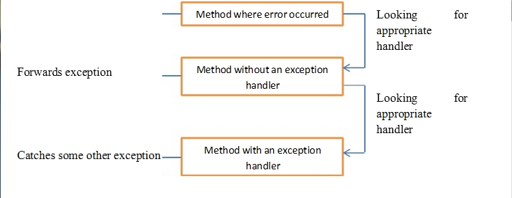
  • Menyediakan mekanisme yang memungkinkan untuk menjalankan kesalahan yang terjadi dalam sebuah metode ke metode yang melakukan pemanggilan metode itu.
  • Menangani berbagai jenis kondisi yang abnormal.

Keyword Exception Handling
1.
Throw

Saat terjadi exception, maka akan terbentuk exception objek dan runtime pada Java akan berjalan untuk melakukan penanganan. Kita dapat melemparkan exception tersebut secara eksplisit dengan keyword throw.

Syntax : throw variableObject;

Aliran eksekusi akan segera terhenti setelah pernyataan throw dan pernyataan selanjutnya tidak akan dicapai. Block try terdekat akan diperiksa untuk melihat catch yang cocok dengan tipe instace throwable. Bila benar, blok try akan diperiksa. Bila tidak, blok try selanjutkan akan diperiksa sampai menemukan blok try yang bermasalah.

2.Throws

Digunakan untuk mengenali daftar exception yang mungkin di throw oleh suatu method. Jika tipe exception adalah error atau runtime exception maka aturan ini tidak berlaku karena tidak diharapkan sebagai bagian normal dari kerja program.

Syntax: Type method-name(arg-list) throws exception-listy{}
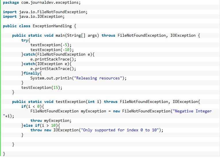
3.Try Catch

Digunakan untuk mengesekusi suatu bagian program, bila muncul kesalahan maka sistem akan melakukan throw suatu exception yang dapat menangkap berdasarkan tipe exception atau yang diberikan finally dengan penagann default.

Syntax: try { //Code// } catch ( ExceptionName ) { //Code// }

4, Finally

Digunakan untuk membuat blok yang mengikuti blok try. Blok finally akan selalu dieksekusi, tidak peduli exception terjadi atau tidak. Sehingga, menggunakan keyword finally memungkinkan untuk menjalankan langkah akhir yang harus dijalankan tidak peduli apa yang terjadi di bagian protected code.

  1. Checked dan Unchecked Exceptions

Checked exception merupakan exception yang diperiksa oleh Java compiler yang memeriksa keseluruhan program apakah menangkap exception yang terjadi dalam syntax throws. Apabila checked exception tidak ditangkap, maka compiler akan error. Tidak seperti checked exception, unchecked exception tidak berupa compile time checking dalam exception handling dikarenakan pondasi dasar unchecked exception adalah error dan runtime exception.

Exception Keyword

  1. Metode Throwable Class

Terbagi menjadi 5 macam metode:

  1. Public String getMessage(): megembalikan pesan pada saat exception memasuki constructor.
  2. Public String getLocalizedMessage(): subclass dapat overide untuk mendukung pesan spesifik lokal yang disebut sebagai pemanggilan program.
  3. Public synchronized Throwable getCause(): untuk exception yang null
  4. Public String toString(): mengembalikan informasi dan pesan lokal.
  5. Public void printStackTrace: mencetak stack trace.
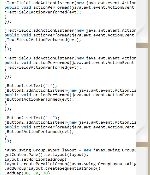
  1. Event Handling

Event handling merupakan suatu konsep penanganan terhadap aksi yang terjadi. Sebagai contoh, jika kita klik buttonklik maka akan ditampilkan sebuah pop up. Hal sederhana ini merupakan contoh dari event handling. Masih banyak berbagai contoh mengenai event handling yang tidak hanya buttonklik saja.

Dalam event handling, terdapat empat bagian penting yang harus diketahui:

  1. Event object merupakan objek yang mendeskripsikan sebuah event yang di trigger oleh event source.
  2. Event handler merupakan method yang menerima event object dan melakukan respon yang sesuai dengan event object.
  3. Event listener merupakan interface yang akan melakukan handle terhadap event yang terjadi. Listener harus diimplementasikan oleh class yang akan melakukan handle terhadap event.
  4. Event source merupakan pembangkit sebuah event object.

Untuk dapat melakukan listener, diperlukan sebuah class yang terdapat pada java.awt.event.*;.

Dengan demikian, event terbagi menjadi beberapa kategori seperti:

  1. Action merupakan interface dari ActionListener dengan method actionPerformed.
  2. Item merupakan interface dari ItemListener dengan method itemStateChange.
  3. Mouse merupakan interface dari MouseListener dengan lima method yaitu:
  4. mouseClicked
  5. mousePressed
  6. mouseReleased
  7. mouseEntered
  8. mouseExited
  9. Mouse motion merupakan interface dari MouseMotionListener dengan method mouseDragged.
  10. Focus merupakan interface dari FocusListener dengan dua method yaitu:
  11. focusGained
  12. focusLast
  13. Window merupakan interface WindowsListener dengan empat method yaitu:
  14. windowClosing
  15. windowOpened
  16. windowActivated
  17. windowDeactived

Setiap event object memiliki tipe event yang berbeda sehingga kita harus menentukan tipe event sebelum menentukan jenis interface listener karena tipe event memiliki jenis interface yang bersesuaian.

Berikut merupakan tipe event yang ada di bahasa Java:

  1. ActionEvent
  2. ItemEvent
  3. WindowEvent
  4. ContainerEvent
  5. ComponenEvent
  6. FocusEvent
  7. TextEvent
  8. KeyEvent
  9. MouseEvent
  10. AdjustmentEvent

Berikut juga merupakan interface listener yang terdapat pada bahasa Java:

  1. ActionListener: menerima event action pada suatu komponen.
  2. ItemListener: menerima item event.
  3. WindowListener: menerima aksi atas perubahan windows.
  4. ContainerListener
  5. ComponenListener
  6. FocusListener: menerima keyboard focus events pada sebuah komponen.
  7. TextListener
  8. KeyListener: keyboard event dihasilkan ketika sebuah key ditekan, dilepas, atau diketik.
  9. MouseListener: menerima mouse event pada suatu komponen.
  10. MouseMotionListener: menerima mouse motion event.
  11. AdjustmentListener: bereaksi terhadap perubahan yang terjadi.

Berikut merupakan tahapan mengenai cara melakukan event handling dalam Java:

  1. Deklarasikan class yang akan melakukan event handle yang terjadi dan tuliskan kode yang menyatakan class tersebut mengimplementasikan interface listener.
  2. Event source mendaftarkan sebuah listener melalui method add<type>Listener
  3. Kode yang mengimplementasikan method pada interface listener pada class akan melakukan event handle.

Contoh Event Handle

Posted in Uncategorized | 152 Comments

session 10(Concurrency)

In programming, these situations are encountered:

  • When two processes are assigned to different cores on a machine by the kernel, and both cores execute the process instructions at the same time.
  • When more connections arrive before earlier connections are finished, and need to be handled immediately.

More generally, it’s when we need to handle multiple tasks at about the same time.

That’s it. That’s all concurrency is. Parallel execution is when two tasks start at the same time, making it a special case of concurrent execution.

Why Does The Ability to Handle Concurrency Matter?

Because concurrency leads to several issues:

  • How do you maintain, store and ensure the consistency of information between independent tasks that require the ability to read and write to shared information?
  • How do you adequately allocate a finite number of resources to handle a potentially monotonically increasing number of jobs to finish?
  • How do you distribute novel information across existing services concurrently handling work at the same time?

A kernel is a microcosm of all these conundrums:

  • It must be able to prevent memory corruption by dynamically assigning and reassigning virtual memory addresses to programs when they require it while maintaining a mapping from virtual memory to physical memory.
  • It must allocate and assign a finite number of cores to multiple programs, often utilising scheduling algorithms to allow the same core to work on multiple programs in the same unit of time to maximise utilisation.
  • It must be able to communicate with programs in the event of unexpected issues e.g. when a hardware interrupt occurs that requires the program to quit immediately.

But these issues are not limited to the kernel:

  • A distributed database may handle several hundred thousand reads and writes at the same time. It is of interest to ensure that each read reflects the state of the database after the writes received at the same time were processed.
  • A data ingestion pipeline may require several processes to communicate with each other, often to synchronise their executions if they’re taking place on machines with a different clock frequency.
  • A content delivery network must be able to handle the unexpected loss of a server or the addition of brand new ones without compromising the integrity of the information, as they may be launched at any moment to handle increased load such as during a DDoS attack).

Approaches to Handling Concurrency

From a very high-level perspective, there are really only a few tactics for safely dealing with tasks that must be run concurrently:

  • Launch many workers, and have them read, as well as write, information from the same place for all to see.

    This is like hiring workers and having them all come up to a bulletin board to learn of new changes and update it with discoveries.

    This approach often runs into race conditions: what happens if one worker tries to read the bulletin board at the same time someone is trying to write on it? Should they wait for them to finish, or should they get back to work right away? What if they both try to write at the same time over each other, even though the overwritten information is more important?

    Computers deal with these situations by either

    • employing the use of thread-safe structures – effectively, all workers must stand in a queue if they want to read or write. This is one of the oldest solutions out there to this problem, and features heavily in Python, C++, and Java.
    • requiring that a shared resource never have writes written to it. This is called guaranteeing immutability, and is fashionable in modern server-side Javascript development as well as being a design feature of the programming language Rust.
  • Launch many workers, and have them update any other worker that requires information.

    This is like hiring workers and having them go up to other workers and tell them that they’re done. For programs that require a lot of cooperation, this means a lot of messages passed. For programs that have many workers at many stages, it is ideal for intimating other stages that one stage is done.

    This is also the concurrency model espoused by many languages, such as Eralng and Scala, and is referred to as the actor model or message-passing concurrency.

  • Launch one very, very, very good worker and have them split their time effectively on tasks.

    This is a design staple of web servers like Nginx and Node.js, or in-memory stores like Redis, where they handle multiple incoming tasks with exactly one worker.

    Exactly one worker handles incoming tasks. This worker is able to effectively divide its time very effectively between working on an existing task and beginning a new work, so that it “seems” like it’s actually doing both tasks at the same time but really isn’t.

    It immediately sidesteps all the problems associated with multiple people, but, well, even one worker can only do so much.

Posted in Uncategorized | 3 Comments

session 9(object oriented programing)

In this Session IX : Object Oriented Programming there are 5 sub topics:

  • Introduction
  • Object-Oriented Programming
  • Design Issues for Object-Oriented Languages
  • Support for Object-Oriented Programming in C++
  • Implementation of Object-Oriented Constructs


Introduction

Languages that support object-oriented programming now are firmly entrenched in the mainstream. From COBOL to LISP, including virtually every language in between, dialects that support object-oriented programming have appeared. C++, Objective-C, and Ada 95 support procedural and data-oriented programming, in addition to object-oriented programming. Newer languages do not support other paradigms but use their imperative structures (e.g., Java and C#), some are pure OOP language (e.g., Smalltalk & Ruby)

Object-Oriented Programming

There are three major language features:

–Abstract data types : already discussed in session VIII

–Inheritance

–Polymorphism

Inheritance

Inheritance is the central theme in OOP. Inheritance offers a solution to both the modification problem posed by abstract data type reuse and the program organization problem. If a new abstract data type can inherit the data and functionality of some existing type, and is also allowed to modify some of those entities and add new entities, reuse is greatly facilitated without requiring changes to the reused abstract data type. Programmers can begin with an existing abstract data type and design a modified descendant of it to fit a new problem requirement. Furthermore, inheritance provides a framework for the definition of hierarchies of related classes that can reflect the descendant relationships in the problem space.

  • Inheritance can be complicated by access controls to encapsulated entities
    • A class can hide entities from its subclasses
    • A class can hide entities from its clients
    • A class can also hide entities for its clients while allowing its subclasses to see them
  • Besides inheriting methods as is, a class can modify an inherited method
    • The new one overrides the inherited one
    • The method in the parent is overriden

There are 3 ways a class can differ from its parent:

  1. The parent class can define some of its variables or methods to have private access, which means they will not be visible in the subclass
  2. The subclass can add variables and/or methods to those inherited from the parent
  3. The subclass can modify the behavior of one or more of its inherited methods.

There are two kinds of variables in a class:

  • Class variables – one/class
  • Instance variables – one/object

There are two kinds of methods in a class:

  • Class methods – accept messages to the class
  • Instance methods – accept messages to objects

One disadvantage of inheritance for reuse is it creates interdependencies among classes that complicate maintenance

Dynamic Binding (Polymorphism)

Polymorphism is a natural part of any object-oriented language that is statically typed. In a sense, polymorphism makes a statically typed language a little bit dynamically typed, where the little bit is in some bindings of method calls to methods. The type of a polymorphic variable is indeed dynamic. A polymorphic variable can be defined in a class that is able to reference (or point to) objects of the class and objects of any of its descendants. When a class hierarchy includes classes that override methods and such methods are called through a polymorphic variable, the binding to the correct method will be dynamic. One purpose of dynamic binding is to allow software systems to be more easily extended during both development and maintenance.


Support for Object-Oriented Programming in C++

To main backward compatibility with C, C++ retains the type system of C and adds classes to it. Therefore, C++ has both traditional imperative-language types and the class structure of an object-oriented language. It supports methods, as well as functions that are not related to specific classes. This makes it a hybrid language, supporting both procedural programming and object- oriented programming.

A C++ class can be derived from an existing class, which is then its parent, or base, class. Unlike Smalltalk and most other languages that support object- oriented programming, a C++ class can also be stand-alone, without a superclass. All C++ objects must be initialized before they are used. Therefore, all C++ classes include at least one constructor method that initializes the data members of the new object. Constructor methods are implicitly called when an object is created. If any of the data members are pointers to heap-allocated data, the constructor allocates that storage.

All of the member functions we have defined thus far are statically bound; that is, a call to one of them is statically bound to a function definition. A C++ object could be manipulated through a value variable, rather than a pointer or a reference. (Such an object would be static or stack dynamic.) However, in that case, the object’s type is known and static, so dynamic binding is not needed. On the other hand, a pointer variable that has the type of a base class can be used to point to any heap-dynamic objects of any class publicly derived from that base class, making it a polymorphic variable. Publicly derived subclasses are subtypes if none of the members of the base class are private. Privately derived subclasses are never subtypes. A pointer to a base class cannot be used to reference a method in a subclass that is not a subtype.

Implementation of Object-Oriented Constructs

There are at least two parts of language support for object-oriented programming that pose interesting questions for language implementers: storage structures for instance variables and the dynamic bindings of messages to methods.

  • Storage structures for instance variablesIn C++, classes are defined as extensions of C’s record structures—structs. This similarity suggests a storage structure for the instance variables of class instances—that of a record. This form of this structure is called a class instance record (CIR). The structure of a CIR is static, so it is built at compile time and used as a template for the creation of the data of class instances. Every class has its own CIR. When a derivation takes place, the CIR for the subclass is a copy of that of the parent class, with entries for the new instance variables added at the end.
  • Dynamic binding of messages to methodsMethods in a class that are statically bound need not be involved in the CIR for the class. However, methods that will be dynamically bound must have entries in this structure. Such entries could simply have a pointer to the code of the method, which must be set at object creation time. Calls to a method could then be connected to the corresponding code through this pointer in the CIR. The drawback to this technique is that every instance would need to store pointers to all dynamically bound methods that could be called from the instance.
Posted in Uncategorized | 1 Comment

session 8 (abstract data type)

Abstract Data Types or ADT is a user-defined data types.

Also, can be explained this way, we have a primitive data types (e.g. char, float). But sometimes we want to store the data as one (e.g. Names, Address, telephone number). We then can declare an abstract data types to handle that.

In an ADT, we can create our own data types using the existing primitive data types or even object, and name the ADT whatever we want.

The class is the encapsulation device

  • A class is a type
  • All of the class instances of a class share a single copy of the member functions
  • Each instance of a class has its own copy of the class data members
  • Instances can be static, stack dynamic, or heap dynamic
  • Information Hiding

o   Private clause for hidden entities

o   Public clause for interface entities

o   Protected clause for inheritance

  • Constructors:

o   Functions to initialize the data members of instances (they do not create the objects)

o   May also allocate storage if part of the object is heap-dynamic

o   Can include parameters to provide parameterization of the objects

o   Implicitly called when an instance is created

o   Can be explicitly called

o   Name is the same as the class name

  • Destructors

o   Functions to cleanup after an instance is destroyed; usually just to reclaim heap storage

o   Implicitly called when the object’s lifetime ends

o   Can be explicitly called

o   Name is the class name, preceded by a tilde (~)

  • Example in C++

class Stack {

private:

int *stackPtr, maxLen, topPtr;

public:

Stack() { // a constructor

stackPtr = new int [100];

maxLen = 99;

topPtr = -1;

};

~Stack () {delete [] stackPtr;};

void push (int number) {

if (topSub == maxLen)

cerr << ″Error in push – stack is full\n″;

else stackPtr[++topSub] = number;

};

void pop () {…};

int top () {…};

int empty () {…};

}

  • Friend functions or classes – to provide access to private members to some unrelated units or functions
  • Necessary in C++

Encapsulation Constructs

  • Large programs have two special needs:

o   Some means of organization, other than simply division into subprograms

o   Some means of partial compilation (compilation units that are smaller than the whole program)

  • Obvious solution: a grouping of subprograms that are logically related into a unit that can be separately compiled (compilation units)
  • Such collections are called encapsulation

Nested Subprograms

  • Organizing programs by nesting subprogram definitions inside the logically larger subprograms that use them
  • Nested subprograms are supported in Ada, Fortran 95+, Python, JavaScript, and Ruby

Encapsulation in C

  • Files containing one or more subprograms can be independently compiled
  • The interface is placed in a header file
  • Problem: the linker does not check types between a header and associated implementation
  • #include preprocessor specification – used to include header files in applications

Encapsulation in C++

  • Can define header and code files, similar to those of C
  • Or, classes can be used for encapsulation

o   The class is used as the interface (prototypes)

o   The member definitions are defined in a separate file

  • Friends provide a way to grant access to private members of a class

Naming Encapsulations

  • Large programs define many global names; need a way to divide into logical groupings
  • A naming encapsulation is used to create a new scope for names
  • C++ Namespaces

o   Can place each library in its own namespace and qualify names used outside with the namespace

o   C# also includes namespaces

  • Java Packages

o   Packages can contain more than one class definition; classes in a package are partial friends

o   Clients of a package can use fully qualified name or use the import declaration

  • Ruby classes are name encapsulations, but Ruby also has modules
  • Typically encapsulate collections of constants and methods
  • Modules cannot be instantiated or subclassed, and they cannot define variables
  • Methods defined in a module must include the module’s name
  • Access to the contents of a module is requested with the require method
Posted in Uncategorized | 1 Comment

session 7 (expression and assignment statements)

Introduction ƒ Expressions are the fundamental means of specifying computations in a programming language. ƒ To understand expression evaluation, need to be familiar with the orders of operator and operand evaluation. ƒ Essence of imperative languages is dominant role of assignment statements.
Arithmetic Expressions ƒ Their evaluation was one of the motivations for the development of the first programming languages. ƒ Most of the characteristics of arithmetic expressions in programming languages were inherited from conventions that had evolved in math. ƒ Arithmetic expressions consist of operators, operands, parentheses, and function calls. ƒ The operators can be unary, or binary. C-based languages include a ternary operator, which has three operands (conditional expression). ƒ The purpose of an arithmetic expression is to specify an arithmetic computation. ƒ An implementation of such a computation must cause two actions: o Fetching the operands from memory o Executing the arithmetic operations on those operands. ƒ Design issues for arithmetic expressions: 1. What are the operator precedence rules? 2. What are the operator associativity rules? 3. What is the order of operand evaluation? 4. Are there restrictions on operand evaluation side effects? 5. Does the language allow user-defined operator overloading? 6. What mode mixing is allowed in expressions?
Operator Evaluation Order 1. Precedence ƒ The operator precedence rules for expression evaluation define the order in which “adjacent” operators of different precedence levels are evaluated (“adjacent” means they are separated by at most one operand). ƒ Typical precedence levels: 1. parentheses 2. unary operators 3. ** (if the language supports it) 4. *, /
5. +, – ƒ Many languages also include unary versions of addition and subtraction. ƒ Unary addition (+) is called the identity operator because it usually has no associated operation and thus has no effect on its operand. ƒ In Java, unary plus actually does have an effect when its operand is short or byte. An implicit conversion of short and byte operands to int type takes place. ƒ Unary minus operator (-) Ex:

A + (- B) * C // is legal A + – B * C // is illegal

2. Associativity ƒ The operator associativity rules for expression evaluation define the order in which adjacent operators with the same precedence level are evaluated. An operator can be either left or right associative. ƒ Typical associativity rules: o Left to right, except **, which is right to left o Sometimes unary operators associate right to left (e.g., FORTRAN) ƒ Ex: (Java)

a – b + c // left to right

ƒ Ex: (Fortran)

A ** B ** C // right to left

(A ** B) ** C // In Ada it must be parenthesized

Language Associativity Rule FORTRAN Left: * / + – Right: ** C-BASED LANGUAGES Left: * / % binary + binary – Right: ++ — unary – unary + ADA Left: all except ** Non-associative: **

ƒ APL is different; all operators have equal precedence and all operators associate right to left. ƒ Ex:

A X B + C // A = 3, B = 4, C = 5 Î 27

ƒ Precedence and associativity rules can be overridden with parentheses.

3. Parentheses ƒ Programmers can alter the precedence and associativity rules by placing parentheses in expressions. ƒ A parenthesized part of an expression has precedence over its adjacent un-parenthesized parts. ƒ Ex:

(A + B) * C

4. Conditional Expressions ƒ Sometimes if-then-else statements are used to perform a conditional expression assignment.

if (count == 0) average = 0; else average = sum / count;

ƒ In the C-based languages, this can be specified more conveniently in an assignment statement using a conditional expressions. Note that ? is used in conditional expression as a ternary operator (3 operands).

expression_1 ? expression_2 : expression_3

ƒ Ex:

average = (count == 0) ? 0 : sum / count;

Operand evaluation order ƒ The process: 1. Variables: just fetch the value from memory. 2. Constants: sometimes a fetch from memory; sometimes the constant is in the machine language instruction. 3. Parenthesized expressions: evaluate all operands and operators first.

• Side Effects ƒ A side effect of a function, called a functional side effect, occurs when the function changes either one of its parameters or a global variable. ƒ Ex:

a + fun(a)

ƒ If fun does not have the side effect of changing a, then the order of evaluation of the two operands, a and fun(a), has no effect on the value of the expression. ƒ However, if fun changes a, there is an effect. ƒ Ex: Consider the following situation: fun returns the value of its argument divided by 2 and changes its parameter to have the value 20, and:

a = 10; b = a + fun(a);

ƒ If the value of a is returned first (in the expression evaluation process), its value is 10 and the value of the expression is 15. ƒ But if the second is evaluated first, then the value of the first operand is 20 and the value of the expression is 25. ƒ The following shows a C program which illustrate the same problem.

int a = 5; int fun1() { a = 17; return 3; } void fun2() { a = a + fun1(); // C language a = 20; Java a = 8 } void main() { fun2(); }

ƒ The value computed for a in fun2 depends on the order of evaluation of the operands in the expression a + fun1(). The value of a will be either 8 or 20. ƒ Two possible solutions: 1. Write the language definition to disallow functional side effects o No two-way parameters in functions. o No non-local references in functions. o Advantage: it works! o Disadvantage: Programmers want the flexibility of two-way parameters (what about C?) and non-local references. 2. Write the language definition to demand that operand evaluation order be fixed o Disadvantage: limits some compiler optimizations

Java guarantees that operands are evaluated in left-to-right order, eliminating this problem. // C language a = 20; Java a = 8

Assignment Statements
Simple Assignments ƒ The C-based languages use == as the equality relational operator to avoid confusion with their assignment operator. ƒ The operator symbol for assignment: 1. = FORTRAN, BASIC, PL/I, C, C++, Java 2. := ALGOL, Pascal, Ada
Conditional Targets ƒ Ex:

flag ? count 1 : count2 = 0; ⇔ if (flag) count1 = 0; else count2 = 0;
Compound Assignment Operators ƒ A compound assignment operator is a shorthand method of specifying a commonly needed form of assignment. ƒ The form of assignment that can be abbreviated with this technique has the destination var also appearing as the first operand in the expression on the right side, as in

a = a + b

ƒ The syntax of assignment operators that is the catenation of the desired binary operator to the = operator. sum += value; ⇔ sum = sum + value;
Unary Assignment Operators ƒ C-based languages include two special unary operators that are actually abbreviated assignments. ƒ They combine increment and decrement operations with assignments. ƒ The operators ++ and — can be used either in expression or to form standalone single-operator assignment statements. They can appear as prefix operators:

sum = ++ count; ⇔ count = count + 1; sum = count;
ƒ If the same operator is used as a postfix operator:

sum = count ++; ⇔ sum = count; count = count + 1;
Assignment as an Expression

ƒ This design treats the assignment operator much like any other binary operator, except that it has the side effect of changing its left operand. ƒ Ex:

while ((ch = getchar())!=EOF) {…} // why ( ) around assignment?

ƒ The assignment statement must be parenthesized because the precedence of the assignment operator is lower than that of the relational operators. ƒ Disadvantage: Another kind of expression side effect which leads to expressions that are difficult to read and understand. For example

a = b + (c = d / b++) – 1

denotes the instructions Assign b to temp Assign b + 1 to b Assign d / temp to c Assign b + c to temp Assign temp – 1 to a

ƒ There is a loss of error detection in the C design of the assignment operation that frequently leads to program errors.

if (x = y) …

instead of

if (x == y) …

Mixed-Mode Assignment ƒ In FORTRAN, C, and C++, any numeric value can be assigned to any numeric scalar variable; whatever conversion is necessary is done. ƒ In Pascal, integers can be assigned to reals, but reals cannot be assigned to integers (the programmer must specify whether the conversion from real to integer is truncated or rounded.) ƒ In Java, only widening assignment coercions are done. ƒ In Ada, there is no assignment coercion. ƒ In all languages that allow mixed-mode assignment, the coercion takes place only after the right side expression has been evaluated. For example, consider the following code:

int a, b; float c; … c = a / b;

Because c is float, the values of a and b could be coerced to float before the division, which could produce a different value for c than if the coercion were delayed (for example, if a were 2 and b were 3).

Posted in Uncategorized | 1 Comment

session 6 (data types)

Data Types

Every value in Rust is of a certain type, which tells Rust what kind of data is being specified so it knows how to work with that data. In this section, we’ll look at a number of types that are built into the language. We split the types into two subsets: scalar and compound.

Throughout this section, keep in mind that Rust is a statically typed language, which means that it must know the types of all variables at compile time. The compiler can usually infer what type we want to use based on the value and how we use it. In cases when many types are possible, such as when we converted a String to a numeric type using parse in Chapter 2, we must add a type annotation, like this:


let guess: u32 = "42".parse().expect("Not a number!");

If we don’t add the type annotation here, Rust will display the following error, which means the compiler needs more information from us to know which possible type we want to use:

error[E0282]: type annotations needed
 --> src/main.rs:2:9
  |
2 |     let guess = "42".parse().expect("Not a number!");
  |         ^^^^^
  |         |
  |         cannot infer type for `_`
  |         consider giving `guess` a type

You’ll see different type annotations as we discuss the various data types.

Scalar Types

A scalar type represents a single value. Rust has four primary scalar types: integers, floating-point numbers, booleans, and characters. You’ll likely recognize these from other programming languages, but let’s jump into how they work in Rust.

Integer Types

An integer is a number without a fractional component. We used one integer type earlier in this chapter, the u32 type. This type declaration indicates that the value it’s associated with should be an unsigned integer (signed integer types start with i instead of u) that takes up 32 bits of space. Table 3-1 shows the built-in integer types in Rust. Each variant in the Signed and Unsigned columns (for example, i16) can be used to declare the type of an integer value.

Table 3-1: Integer Types in Rust

Length Signed Unsigned
8-bit i8 u8
16-bit i16 u16
32-bit i32 u32
64-bit i64 u64
arch isize usize

Each variant can be either signed or unsigned and has an explicit size. Signed and unsigned refers to whether it’s possible for the number to be negative or positive; in other words, whether the number needs to have a sign with it (signed) or whether it will only ever be positive and can therefore be represented without a sign (unsigned). It’s like writing numbers on paper: when the sign matters, a number is shown with a plus sign or a minus sign; however, when it’s safe to assume the number is positive, it’s shown with no sign. Signed numbers are stored using two’s complement representation (if you’re unsure what this is, you can search for it online; an explanation is outside the scope of this book).

Each signed variant can store numbers from -(2n – 1) to 2n – 1 – 1 inclusive, where n is the number of bits that variant uses. So an i8 can store numbers from -(27) to 27 – 1, which equals -128 to 127. Unsigned variants can store numbers from 0 to 2n – 1, so a u8 can store numbers from 0 to 28 – 1, which equals 0 to 255.

Additionally, the isize and usize types depend on the kind of computer your program is running on: 64-bits if you’re on a 64-bit architecture and 32-bits if you’re on a 32-bit architecture.

You can write integer literals in any of the forms shown in Table 3-2. Note that all number literals except the byte literal allow a type suffix, such as 57u8, and _ as a visual separator, such as 1_000.

Table 3-2: Integer Literals in Rust

Number literals Example
Decimal 98_222
Hex 0xff
Octal 0o77
Binary 0b1111_0000
Byte (u8 only) b'A'

So how do you know which type of integer to use? If you’re unsure, Rust’s defaults are generally good choices, and integer types default to i32: it’s generally the fastest, even on 64-bit systems. The primary situation in which you’d use isize or usize is when indexing some sort of collection.

Floating-Point Types

Rust also has two primitive types for floating-point numbers, which are numbers with decimal points. Rust’s floating-point types are f32 and f64, which are 32 bits and 64 bits in size, respectively. The default type is f64 because on modern CPUs it’s roughly the same speed as f32 but is capable of more precision.

Here’s an example that shows floating-point numbers in action:

Filename: src/main.rs

fn main() {
    let x = 2.0; // f64

    let y: f32 = 3.0; // f32
}

Floating-point numbers are represented according to the IEEE-754 standard. The f32 type is a single-precision float, and f64 has double precision.

Numeric Operations

Rust supports the usual basic mathematical operations you’d expect for all of the number types: addition, subtraction, multiplication, division, and remainder. The following code shows how you’d use each one in a let statement:

Filename: src/main.rs

fn main() {
    // addition
    let sum = 5 + 10;

    // subtraction
    let difference = 95.5 - 4.3;

    // multiplication
    let product = 4 * 30;

    // division
    let quotient = 56.7 / 32.2;

    // remainder
    let remainder = 43 % 5;
}

Each expression in these statements uses a mathematical operator and evaluates to a single value, which is then bound to a variable. Appendix B contains a list of all operators that Rust provides.

The Boolean Type

As in most other programming languages, a boolean type in Rust has two possible values: true and false. The boolean type in Rust is specified using bool. For example:

Filename: src/main.rs

fn main() {
    let t = true;

    let f: bool = false; // with explicit type annotation
}

The main way to consume boolean values is through conditionals, such as an if expression. We’ll cover how if expressions work in Rust in the “Control Flow” section.

The Character Type

So far we’ve only worked with numbers, but Rust supports letters too. Rust’s char type is the language’s most primitive alphabetic type, and the following code shows one way to use it. Note that the char type is specified with single quotes, as opposed to strings that use double quotes:

Filename: src/main.rs

fn main() {
   let c = 'z';
   let z = 'ℤ';
   let heart_eyed_cat = '😻';
}

Rust’s char type represents a Unicode Scalar Value, which means it can represent a lot more than just ASCII. Accented letters, Chinese/Japanese/Korean ideographs, emoji, and zero width spaces are all valid char types in Rust. Unicode Scalar Values range from U+0000 to U+D7FF and U+E000 to U+10FFFF inclusive. However, a “character” isn’t really a concept in Unicode, so your human intuition for what a “character” is may not match up with what a char is in Rust. We’ll discuss this topic in detail in the “Strings” section in Chapter 8.

Compound Types

Compound types can group multiple values of other types into one type. Rust has two primitive compound types: tuples and arrays.

Grouping Values into Tuples

A tuple is a general way of grouping together some number of other values with a variety of types into one compound type.

We create a tuple by writing a comma-separated list of values inside parentheses. Each position in the tuple has a type, and the types of the different values in the tuple don’t have to be the same. We’ve added optional type annotations in this example:

Filename: src/main.rs

fn main() {
    let tup: (i32, f64, u8) = (500, 6.4, 1);
}

The variable tup binds to the entire tuple, since a tuple is considered a single compound element. To get the individual values out of a tuple, we can use pattern matching to destructure a tuple value, like this:

Filename: src/main.rs

fn main() {
    let tup = (500, 6.4, 1);

    let (x, y, z) = tup;

    println!("The value of y is: {}", y);
}

This program first creates a tuple and binds it to the variable tup. It then uses a pattern with let to take tup and turn it into three separate variables, x, y, and z. This is called destructuring, because it breaks the single tuple into three parts. Finally, the program prints the value of y, which is 6.4.

In addition to destructuring through pattern matching, we can also access a tuple element directly by using a period (.) followed by the index of the value we want to access. For example:

Filename: src/main.rs

fn main() {
    let x: (i32, f64, u8) = (500, 6.4, 1);

    let five_hundred = x.0;

    let six_point_four = x.1;

    let one = x.2;
}

This program creates a tuple, x, and then makes new variables for each element by using their index. As with most programming languages, the first index in a tuple is 0.

Arrays

Another way to have a collection of multiple values is with an array. Unlike a tuple, every element of an array must have the same type. Arrays in Rust are different than arrays in some other languages because arrays in Rust have a fixed length: once declared, they cannot grow or shrink in size.

In Rust, the values going into an array are written as a comma-separated list inside square brackets:

Filename: src/main.rs

fn main() {
    let a = [1, 2, 3, 4, 5];
}

Arrays are useful when you want your data allocated on the stack rather than the heap (we will discuss the stack and the heap more in Chapter 4), or when you want to ensure you always have a fixed number of elements. They aren’t as flexible as the vector type, though. The vector type is a similar collection type provided by the standard library that is allowed to grow or shrink in size. If you’re unsure whether to use an array or a vector, you should probably use a vector: Chapter 8 discusses vectors in more detail.

An example of when you might want to use an array rather than a vector is in a program that needs to know the names of the months of the year. It’s very unlikely that such a program will need to add or remove months, so you can use an array because you know it will always contain 12 items:


let months = ["January", "February", "March", "April", "May", "June", "July",
              "August", "September", "October", "November", "December"];
Accessing Array Elements

An array is a single chunk of memory allocated on the stack. We can access elements of an array using indexing, like this:

Filename: src/main.rs

fn main() {
    let a = [1, 2, 3, 4, 5];

    let first = a[0];
    let second = a[1];
}

In this example, the variable named first will get the value 1, because that is the value at index [0] in the array. The variable named second will get the value 2 from index [1] in the array.

Invalid Array Element Access

What happens if we try to access an element of an array that is past the end of the array? Say we change the example to the following:

Filename: src/main.rs

fn main() {
    let a = [1, 2, 3, 4, 5];
    let index = 10;

    let element = a[index];

    println!("The value of element is: {}", element);
}

Running this code using cargo run produces the following result:

$ cargo run
   Compiling arrays v0.1.0 (file:///projects/arrays)
    Finished dev [unoptimized + debuginfo] target(s) in 0.31 secs
     Running `target/debug/arrays`
thread '<main>' panicked at 'index out of bounds: the len is 5 but the index is
 10', src/main.rs:6
note: Run with `RUST_BACKTRACE=1` for a backtrace.

The compilation didn’t produce any errors, but the program results in a runtime error and didn’t exit successfully. When you attempt to access an element using indexing, Rust will check that the index you’ve specified is less than the array length. If the index is greater than the length, Rust will panic, which is the term Rust uses when a program exits with an error.

This is the first example of Rust’s safety principles in action. In many low-level languages, this kind of check is not done, and when you provide an incorrect index, invalid memory can be accessed. Rust protects you against this kind of error by immediately exiting instead of allowing the memory access and continuing. Chapter 9 discusses more of Rust’s error handling.

Posted in Uncategorized | 1 Comment

session 5 (Names, Scopes, BIndings)

Names, Scopes, and Bindings


  1. Definitions
    1. Name: Identifiers that allow us to refer to variables, constants, functions, types, operations, and so on
    2. Binding: An association of a name with an object
    3. Scope: The lifetime of a binding of a name to an object
    4. Referencing environment: The complete set of bindings in effect at a certain point in a program
  2. Binding Times
    1. Language design time: The syntax and semantics of a language are typically set at language design time. Examples would be the control constructs, how variable declarations are written, whether static or dynamic scoping is used.
    2. Language implementation time: Most language manuals leave a variety of issues to the discretion of the language implementor. Typical examples might be the precision (number of bits) of the fundamental types, the organization and maximum sizes of the stack and the heap, and the handling of run-time exceptions, such as arithmetic overflow.
    3. Compile time: Compiler associates names with objects, for example, a type with a variable or the layout of a stack allocated object with a variable.
    4. Link time: References to functions may not be resolved until separate .o files are compiled together. Then a placeholder reference can be replaced with an “address” (actually an offset from a relocation register)
    5. Load time: A program is actually assigned physical memory when it executes
    6. Run time: Binding is delayed until run-time, such as dynamic typing in interpreted languages (the type of a variable cannot be determined until it is assigned a value in dynamic typing), the assignment of a heap-allocated object to a pointer variable, or the binding of a virtual method to a function call
    7. Static vs dynamic binding
      1. Static binding is any binding that occurs prior to run-time (either compiler or link time)
      2. Dynamic binding is any binding that occurs at run-time (either load or run time)
    8. Earlier binding decisions are associated with faster code (static typing), whereas later binding decisions are associated with more flexible code (dynamic typing, pointers point to different objects)
  3. Scope Rules: Determine the value of a variable when it is not in the current scope
    1. Types of Scope
      1. Static Scope: Scope can be determined at compile-time, typically by finding a matching declaration in the most closely enclosing block
        1. C/C++ only have the global level and the function level
        2. Some languages, like Python, Ada, or Pascal, allow functions to be nested within other functions (e.g., fig 3.4 and fig 3.5 in the Scott text)
        3. Implemented by maintaining a static link in each frame that points to the “parent” frame, which is the frame of the most recent invocation of the lexically surrounding subroutine. The number of links can be statically determined, so a fixed set of instructions can be emitted to follow the links.
        4. Many languages, including Java, allow nested inner classes, which are a form of static scoping. Each instance of an inner class can access the environment of its enclosing classes. Each inner class maintains a static class link to its “enclosing” object, so that at runtime the class chain can be followed to find a reference to an enclosing instance variable. As with static links, a fixed set of instructions can be emitted to follow the links.
        5. Inheritance is another form of nesting, but in this case scope resolution is done at compile time by following class pointers up the inheritance hierarchy. Since an object’s record is simply a collection of all of its ancestor variables, plus its own variables, the compiler can insert a direct reference to the appropriate variable in the object’s record, rather than requiring a run-time search of the class hierarchy.
        6. Some functional languages and many scripting languages do not require variable declarations in functions, and object-oriented languages do not require variable declarations a long as the reference is to an instance variable. Scripting languages handle undeclared variables in different ways.
          1. Python treats any variable that gets assigned a value as a local variable. A programmer can import a global variable using the global keyword
          2. Perl treats any variable that gets assigned a value as a global variable. A programmer can declare a variable as local using either the my keyword for static scoping (newer and preferred), or the local keyword for dynamic scoping (older and generally not wanted)
      2. Dynamic Scope: Scope cannot be determined until run-time, typically by following stack frames until a matching declaration is found.
        1. The number of links is unknown, so a loop must be used to follow the chain.
        2. Used in older languages, like Lisp, and initially in Perl. Perl now has a way of specifying static scope as well.
        3. Provides a convenient way to allow access to variables without passing parameters, but it can make code difficult to follow when reading it statically and code can break if a new subroutine with the same declaration gets inserted during maintanance
        4. See figure 3.9 in the Scott text for an example of the different outcomes that result when using static versus dynamic scoping
  4. Aliasing
    1. Definition: More than one name refers to the same object (aliasing usually is caused by references or pointers)
    2. Problem for compilers: Interferes with optimization. Here’s an example:
      int a, b;
      int *p, *q;
      
      a = *p
      *q = 3
      b = *p; 
      

      The compiler would like to store the value of *p into a register and then assign this register value to b, without having to reload *p. However, if q refers to the same object as p, then the register value is no longer valid. Unless the compiler can prove that q and p can never point to the same object, the compiler must reload the value of *p.

    3. Languages without aliasing, like Fortran, require pointer-based data structures to be implemented using arrays, which is much more efficient, but less flexible. Arrays have contiguous storage and pre-allocate large blocks of memory, which is what makes them more efficient, plus they do not introduce an aliasing problem.
    4. In C99, you may add the restrict qualifier to a pointer declaration. This qualifier asserts that the object to which the pointer refers has no alias in the current scope.
  5. Overloading Built-in Operators: Some languages, such as C++, provide ways to overload built-in operators, such as + or (). Other languages, such as Java, do not allow operator overloading, on the premise that it makes code difficult to statically read, since the reader cannot know which version of the operator will get called.
    1. Forms of operator overloading
      1. Prefix overloading: The operator is treated as though it belongs to a class and takes a single argument (the first argument is the class). For example, in C++, you might have the following definition for an operator that adds two complex numbers:
        class complex {
            double real, imaginary;
            ...
            public:
               complex operator+(complex &other) {
                   return complex(real + other.real, imaginary + other.imaginary);
        };
        ...
        complex A, B, C;
        C = A + B;  // treated by C++ as C = A.operator+(B)
        
      2. Infix overloading: The operator is declared outside a class and its arguments are all provided in an argument list. This handles situations where a class object might not be the left operand. For example, how would one handle the following case with prefix overloading:
        string lname = "vander zanden";
        string name = "brad" + lname;
        

        An example of infix overloading in C++ that handles the above case might be:

        string operator+(char *operand1, string operand2) {
           return string(operand1) + operand2;
        }
        
        int main() {
          string lname = "vander zanden";
          string name = "brad " + lname;
        }
        
  6. Binding of Referencing Environments: When a subroutine can be passed as a parameter to a function, an issue arises as to whether the referencing environment it uses when it is called is the referencing environment in effect when the subroutine is passed as a parameter, or when the subroutine is actually called. It is called deep binding if the referencing environment is the one in effect when the subroutine is passed as a parameter and shallow binding if it is the one in effect when the subroutine is called. Notice that deep binding corresponds to an early binding of the referencing environment and shallow binding corresponds to a late binding of the referencing environment.
    1. Example: Look at the following C++ pseudo-code and assume that it is dynamically scoped
      class person {
         int age;
      }
      
      int threshold;
      database people;
      
      boolean older_than_threshold(person p) {
          return p.age >= threshold;
      }
      
      void print_person(person p) {
          // call appropriate I/O routines to print person on standard output
          // make use of nonlocal variable line_length to format data in columns
      }
      
      void print_selected_records(database db, procedure predicate, print_routine) {
          int line_length;
         
          if (device_type(stdout) == terminal) 
              line_length = 80
          else  // standard line length on older printers or files
              line_length = 132
          
          foreach person p in db do
              if predicate(p) 
                  print_routine(p)
      }
      
      main {
         threshold = 35;
         print_selected_records(people, older_than_threshold, print_person);
      }
      
      1. shallow binding: you would probably want shallow binding for the print routine, since you would want it to pick up the value of line_length set in print_selected_records
      2. deep binding: you would probably want deep binding for threshold, since it appears that you are trying to alter the value of threshold in main and hoping that that value is used for older_than_threshold
    2. Passing Functions as Parameters
      1. Design Considerations
        1. Statically scoped languages typically use deep binding, since you are usually looking to pick up the static scope, not the dynamic scope of a variable (note that shallow binding is essentially saying that you care about what’s on the stack when the function is called, which is what dynamic scoping is all about)
        2. Dynamically scoped languages typically use shallow binding, since you typically do care about what’s on the stack when the function is called
      2. Implementation
        1. Shallow binding: Trivial–same as dynamic scoping
        2. Deep binding: Need to save the current referencing environment as well as a pointer to the function. The bundle as a whole is referred to as a closure
          1. Statically scoped language: Save a pointer to the function and the static link that S would use right now if it were called in the current context. When S is finally called, we temporarily restore the saved static link, rather than creating a new one. When S follows its static chain to access a nonlocal object, it will find the object instance that was current at the time the closure was created. The instance may not have the value it had at the time the closure was created, but its identity, at least, will reflect the intent of the closure’s creator. Note that you are passing a nested function to a more deeply nested function, so when S is called, the less deeply nested context is further down the stack.
          2. Dynamically scope language: Beyond the scope of this course, although our examples will assume that the closure contains references to variables, rather than copies of the variables’ values. Hence changes made by a function will be to the current value of the variable, not the value in effect when the function was passed as a parameter.
    3. Returning Functions as Return Values
      1. Definitions
        1. First class value: can be returned from a function, passed as a parameter, and assigned to variables (e.g., functions in scripting languages, C, C++, functional languages)
        2. Second class: can be passed as a parameter but not returned from a function or assigned to a variable (e.g., functions in some languages)
        3. Third class: cannot be passed even as a parameter (e.g., a label)
      2. Implementation of closures when nested functions may be returned as a return value (note that this is not a problem for non-nested languages such as C)
        1. Example Problem:
          def plus_x(x):
             return def lambda(y):
                      return x+y
          

          plus_x returns an unnamed function (lambda functions denote unnamed functions in functional languages and have been adopted by scripting languages such as Python). This unnamed function takes y as a parameter, adds it to x, and returns the sum. The problem is that in a normal imperative language, x is reclaimed once plus_x exits, and hence would be undefined when our unnamed function is called. This problem is referred to as unlimited extent. Local variables with unlimited extent cannot be reclaimed. This in turn means they cannot be allocated on the stack but instead must be allocated on the heap.

        2. Functional languages: Functional languages simply allocate local objects on the heap and use garbage collection to reclaim them when they are no longer needed
        3. Imperative languages: Imperative languages like to maintain stack-based allocation and reclamation of local objects, so they may place restrictions on returning nested functions
          1. Languages like C and C++ that do not permit nested functions do not have this problem.
          2. Most other imperative languages, like Module-2 an Module-3, only allow outermost functions to be returned as return values and make nested functions either second or third class values
      3. Mimicing the context of nested functions with object closures: In object-oriented languages, we can encapsulate our function as a method and let the object’s fields hold context for the method. Here’s a Java example for the plus_x problem:
        interface IntFunc {
           int call(int i);
        }
        
        class PlusX implements IntFunc {
           int x;
           public PlusX(int n) { x = n; }
           public int call(int i) { return i + x; }
        }
        ...
        IntFunc f = new PlusX(2);
        System.out.println(f.call(3));  // prints 5
        

        The interface defines an abstract type for objects enclosing a function from integers to integers. Whereas Python would capture the value of x in a function closure, Java captures it in an object-closure (also called a function object or functor).

Posted in Uncategorized | 1 Comment

session 4 (lexical and syntax analysis)

Languages

Languages are a potentially infinite set of strings (sometimes called sentences, which are a sequence of symbols from a given alphabet). The tokens of each sentence are ordered according to some structure.

A grammar is a set of rules that describe a language. Grammars assign structure to a sentence.

An automaton is an algorithm that can recognise (accept) all sentences of a language and reject those which do not belong to it.

Lexical and syntactical analysis can be simplified to a machine that takes in some program code, and then returns syntax errors, parse trees and data structures. We can think of the process of description transformation, where we take some source description, apply a transformation technique and end up with a target description – this is inference mapping between two equivalent languages, where the destination is a machine executable.

Compilers are an important part of computer science, even if you never write a compiler, as the concepts are used regularly, in interpreters, intelligent editors, source code debugging, natural language processing (e.g., for AI) and for things such as XML.

Throughout the years, progress has been made in the field of programming to bring higher and higher levels of abstraction, moving from machine code, to assembler, to high level langauges and now to object orrientation, reusable languages and virtual machines.

Translation Process

LSA only deals with the front-end of the compiler, next year’s module CGO deals with the back-end. The front-end of a compiler only analyses the program, it does not produce code.

From source code, lexical analysis produces tokens, the words in a language, which are then parsed to produce a syntax tree, which checks that tokens conform with the rules of a language. Semantic analysis is then performed on the syntax tree to produce an annotated tree. In addition to this, a literal table, which contains information on the strings and constants used in the program, and a symbol table, which stores information on the identifiers occuring in the program (e.g., variable names, constant names, procedure names, etc), are produced by the various stages of the process. An error handler also exists to catch any errors generated by any stages of the program (e.g., a syntax error by a poorly formed line). The syntax tree forms an intermediate representation of the code structure, and has links to the symbol table.

From the annotated tree, intermediate code generation produces intermediate code (e.g., that suitable for a virtual machine, or pseudo-assembler), and then the final code generation stage produces target code whilst also referring to the literal and symbol table and having another error handler. Optimisation is then applied to the target code. The target code could be assembly and then passed to an assembler, or it could be direct to machine code.

We can consider the front-end as a two stage process, lexical analysis and syntactic analysis.

Lexical Analysis

Lexical analysis is the extraction of individual words or lexemes from an input stream of symbols and passing corresponding tokens back to the parser.

If we consider a statement in a programming language, we need to be able to recognise the small syntactic units (tokens) and pass this information to the parser. We need to also store the various attributes in the symbol or literal tables for later use, e.g., if we have an variable, the tokeniser would generate the token var and then associate the name of the variable with it in the symbol table – in this case, the variable name is the lexeme.

Other roles of the lexical analyser include the removal of whitespace and comments and handling compiler directives (i.e., as a preprocessor).

The tokenisation process takes input and then passes this input through a keyword recogniser, an identifier recogniser, a numeric constant recogniser and a string constant recogniser, each being put in to their own output based on disambiguating rules.

These rules may include “reserved words”, which can not be used as identifiers (common examples include begin, end, void, etc), thus if a string can be either a keyword or an identifier, it is taken to be a keyword. Another common rule is that of maximal munch, where if a string can be interpreted as a single token or a sequence of tokens, the former interpretation is generally assumed

The lexical analysis process starts with a definition of what it means to be a token in the language with regular expressions or grammars, then this is translated to an abstract computational model for recognising tokens (a non-deterministic finite state automaton), which is then translated to an implementable model for recognising the defined tokens (a deterministic finite state automaton) to which optimisations can be made (a minimised DFA).

Syntactic Analysis

Syntactic analysis, or parsing, is needed to determine if the series of tokens given are appropriate in a language – that is, whether or not the sentence has the right shape/form. However, not all syntactically valid sentences are meaningful, further semantic analysis has to be applied for this. For syntactic analysis, context-free grammars and the associated parsing techniques are powerful enough to be used – this overall process is called parsing.

In syntactic analysis, parse trees are used to show the structure of the sentence, but they often contain redundant information due to implicit definitions (e.g., an assignment always has an assignment operator in it, so we can imply that), so syntax trees, which are compact representations are used instead. Trees are recursive structures, which complement CFGs nicely, as these are also recursive (unlike regular expressions).

There are many techniques for parsing algorithms (vs FSA-centred lexical analysis), and the two main classes of algorithm are top-down and bottom-up parsing.

For information about
context free grammars,
see MCS.

Context-free grammars can be represented using Backus-Naur Form (BNF). BNF uses three classes of symbols: non-terminal symbols (phrases) enclosed by brackets <>, terminal symbols (tokens) that stand for themselves, and the metasymbol ::= – is defined to be.

As derivations are ambiguous, a more abstract structure is needed. Parse trees generalise derivations and provide structural information needed by the later stages of compilation.

Parse Trees

Parse trees over a grammar G is a labelled tree with a root node labelled with the start symbol (S), and then internal nodes labelled with non-terminals. Leaf nodes are labelled with terminals or ε. If an internal node is labelled with a non-terminal A, and has n children with labels X1, …, Xn (terminals or non-terminals), then we can say that there is a grammar rule of the form A → X1…Xn. Parse trees also have optional node numbers.


The above parse tree corresponds to a leftmost derivation.

Traversing the tree can be done by three different forms of traversal. In preorder traversal, you visit the root and then do a preorder traversal of each of the children, in in-order traversal, an in-order traversal is done of the left sub-tree, the root is visited, and then an in-order traversal is done of the remaining subtrees. Finally, with postorder traversal, a postorder traversal is done of each of the children and the root visited.

Syntax Trees

Parse trees are often converted into a simplified form known as a syntax tree that eliminates wasteful information from the parse tree.


At this stage, treatment of errors is more difficult than in the scanner (tokeniser), as the scanner may pass problems to the parser (an error token). Error recovery typically isolates the error and continues parsing, and repair can be possible in simple cases. Generating meaningful error messages is important, however this can be difficult as the actual error may be far behind the current input token.

Grammars are ambiguous if there exists a sentence with two different parse trees – this is particularly common in arithmetic expressions – does 3 + 4 × 5 = 23 (the natural interpretation, that is 3 + (4 × 5)) or 35 ((3 + 4) × 5). Ambiguity can be inessential, where the parse trees both give the same syntax tree (typical for associative operations), but still a disambiguation rule is required. However, there is no computable function to remove ambiguity from a grammar, it has to be done by hand, and the ambiguity problem is undecidable. Solutions to this include changing the grammar of the language to remove any ambiguity, or to introduce disambiguation rules.

A common disambiguation rule is precedence, where a precedence cascade is used to group operators in to different precedence levels.

BNF does have limitations as there is no notation for repetition and optionality, nor is there any nesting of alternatives – auxillary non-terminals are used instead, or a rule is expanded. Each rule also has no explicit terminator.

Extended BNF (EBNF) was developed to work around these restrictions. In EBNF, terminals are in double quotes “”, and non-terminals are written without <>. Rules have the form non-terminal = sequence or non-terminal = sequence | … | sequence, and a period . is used as the terminator for each rule. {p} is used for 0 more occurrences of p, [p] stands for 0 or 1 occurances of p and (p|q|r) stands for exactly one of p, q, or r. However, notation for repetition does not fully specify the parse tree (left or right associativity?).

Syntax diagrams can be used for graphical representations of EBNF rules. Non-terminals are represented in a square/rectangular box, and terminals in round/oval boxes. Sequences and choices are represented by arrows, and the whole diagram is labelled with the left-hand side non-terminal. e.g., for factor → (exp) | “number” .


Semantic Analysis

Semantic analysis is needed to check aspects that are not related to the syntactic form, or that are not easily determined during parsing, e.g., type correctness of expressions and declaration prior to use.

Code Generation and Optimisation

Code generation and optimisation exists to generally transform the annotated syntax tree into some form of intermediate code, typically three-address code or code for a virtual machine (e.g., p-code). Some level of optimisation can be applied here. This intermediate code can then be transformed into instructions for the target mahcine and optimised further.

Optimisation is really code improvement, e.g., constant folding (e.g., replace x = 4*4 with x = 16), and also at a target level (e.g., multiplications by powers of 2 replaced by shift level instructions).

Bootstrapping

The idea behind bootstrapping is to write a compiler for a language in a possibly older version or a restricted subset of the language. A “quick and dirty” compiler is then written for that language that runs on some machine, but in a restricted subset or older version.

This new version of the compiler incorporates the latest features of the language and generates highly efficient code, and all changes to the language are represented in the new compiler, so this compiler is used to generate the “real” compiler for target machines.

To bootstrap, we use the quick and dirty compiler to compile the new compiler, and then recompile the new compiler with itself to generate an efficient version.

With bootstrapping, improvements to the source code can be bootstrapped by applying the 2-step process. Porting the compiler to a new host computer only requires changes to the backend of the compiler, so the new compiler becomes the “quick and dirty” compiler for new versions of the language.

If we use the main compiler for porting, this provides a mechanism to quickly generate new compilers for all target machines, and minimises the need to maintain/debug multiple compilers.

Top-Down Parsing

Top down parsing can be broken down into two classes: backtracking parsers, which try to apply a grammar rule and backtrack if it fails; and predictive parsers, which try to predict the next nonterminal in the input using one or more tokens lookahead. Backtracking parsers can handle a larger class of grammars, but predictive parsers are faster. We look at predictive parsers in this module.

In this module, we look at two classes of predictive parsers: recursive-descent parsers, which are quite versatile and appropriate for a hand-written parser, and were the first type of parser to be developed; and, LL(1) parsing – left-to-right, leftmost derivation, 1 symbol lookahead, a type of parser which is no longer in use. It does demonstrate parsing using a stack, and helps to formalise the problems with recursive descent. There is a more general class of LL(k) parsers.

Recursive Descent

The basic idea here is that each nonterminal is recognised by a procedure. This choice corresponds to a case or if statement. Strings of terminals and nonterminals within a choice match the input and calls to other procedures. Recursive descent has a one token lookahead, from which the choice of appropriate matching procedure is made.

The code for recursive descent follows the EBNF form of the grammar rule, however the procedures must not use left recursion, which will cause the choice to call a matching procedure in an infinite loop.

There are problems with recursive descent, such as converting BNF rules to EBNF, ambiguity in choice and empty productions (must look on further at tokens that can appear after the current non-terminal). We could also consider adding some form of early error detection, so time is not wasted deriving non-terminals if the lookahead token is not a legal symbol.

Therefore, we can improve recursive descent by defining a set First(α) as the set of tokens that can legally begin α, and a set Follow(A) as the set of tokens that can legally come after the nonterminal A. We can then use First(α) and First(β) to decide between A → α and A → β, and then use Follow(A) to decide whether or not A → ε can be applied.

LL(1) Parsing

LL(1) parsing is top-down parsing using a stack as the memory. At the beginning, the start symbol is put onto the stack, and then two basic actions are available: Generate, which replaces a nonterminal A at the top of the stack by string α using the grammar rule A → α; and Match, which matches a token on the top of the stack with the next input token (and, in case of success, pop both). The appropriate action is selected using a parsing table.

With the LL(1) parsing table, when a token is at the top of the stack, there is either a successful match or an error (no ambiguity). When there is a nonterminal A at the top, a lookahead is used to choose a production to replace A.

The LL(1) parsing table is created by starting with an empty table, and then for all table entries, the production choice A → α is added to the table entry M[A,a] if there is a derivation α ├* aβ where a is a token or there are derivations α ├* ε and S$ ├* βAaγ, where S is that start symbol and a is a token (including $). Any entries that are now empty represent errors.

A grammar is an LL(1) grammar if the associate LL(1) parsing table has at most one production in each table entry. A LL(1) grammar is never ambiguous, so if a grammar is ambiguous, disambiguating rules can be used in simple cases. Some consequences of this are for rules of the form A → α | β, then α and β can not derive strings beginning with the same token a and at most one of α or β can derive ε.

With LL(1) parsing, the list of generated actions match the steps in a leftmost derivation. Each node can be constructed as terminals, or nonterminals are pushed onto the stack. If the parser is not used as a recogniser, then the stack should contain pointers to tree nodes. LL(1) parsing has to generate a syntax tree.

In LL(1) parsing, left recursion and choice are still problematic in similar ways to that of recursive descent parsing. EBNF will not help, so it’s easier to keep the grammar as BNF. Instead, two techniques can be used: left recursion removal and left factoring. This is not a foolproof solution, but it usually helps and it can be automated.

In the case of a simple immediate left recursion of the form A → Aα | β, where α and β are strings and β does not begin with A, then we can rewrite this rule into two grammar rules: A → βA′, A′ → αA′ | ε. The first rule generates β and then generates {α} using right recursion.

For indirect left recursion of the form A → Bβ1 | …, B → Aα1, then a cycle (a derivation of the form A ├ α ├* A) can occur. The algorithm can only work if a grammar has no cycles or ε-productions.

Left recursion removal does not change the language, but it does change the grammar and parse trees, so we now have the new problem of keeping the correct associativity in the syntax tree. If you use the parse tree directly to get the syntax tree, then values need to be passed from parent to child.

If two or more grammar choices share a common prefix string (e.g., A → αβ | αγ), then left factoring can be used. We can factor out the longest possible α and split it into two rules: A → αA′, A′ → β | γ.

To construct a syntax tree in LL(1) parsing, it takes an extra stack to manipulate the syntax tree nodes. Additional symbols are needed in the grammar rules to provide synchronisation between the two stacks, and the usual way of doing this is using the hash (#). In the example of a grammar representing arithmetic operations, the # tells the parser that the second argument has just been seen, so it should be added to the first one.

First and Follow Sets

To construct a First set, there are rules we can follow:

  • If x is a terminal, then First(x) = {x} (and First(ε) = {ε})
  • For a nonterminal A with the production rules A → β1 | … | βn, First(A) = First(β1) ∪ … ∪ First(βn)
  • For a rule of the form A → X1X2…Xn, First(A) = (First(X1) ∪ … ∪ First(Xk)) – {ε}, where ε ∈ First(Xj),j = 1..(k – 1) and ε ∉ First(Xk, i.e., where the first non-nullable symbol X symbol is Xk.

Therefore, the First(w) set consists of the set of terminals that begin strings derived from w (and also contains ε if w can generate ε).

To construct Follow sets, we can say that if A is a non-terminal, then Follow(A) is the set of all terminals that can follow A in any sentential form (derived from S).

  • If A is the start symbol, then the end marker $ ∈ Follow(A)
  • For a production rule of the form B → αAβ, everything in First(β) is placed in Follow(A) except ε.
  • If there is a production B → αA, or a production B → αAβ where First(β) contains ε, then Follow(A) containts Follow(B).

A final issue to consider is how to deal with errors in the parsing stage. In recursive descent parsers, a panic mode exists where each procedure declares a set of synchronising tokens, and when confused, input tokens are skipped (scan ahead) until one of the synchronising sets of tokens are seen and you can continue parsing. In LL(1) parsers, sets of synchronising tokens are kept in an additional stack or built directly into the parsing table.

Posted in Uncategorized | 1 Comment

session 3(describing syntax and semantics)

INTRODUCTION

  • The study of programming languages can be divided into the examination of syntax and semantics
  • Syntax – is the form of expressions, statements, and program units
  • Semantics – is the meaning of those expressions, statements, and program units
  • In a well-designed programming language, semantics should follow directly from syntax
  • Describing syntax is easier than describing semantics

THE GENERAL PROBLEM OF DESCRIBING SYNTAX


  • Lexemes – the lowest level of syntactic unit
  • The lexemes of a programming language include its identifiers, literals, operators and special words
  • Token of a language is a category of its lexemes


LANGUAGE RECOGNIZERS


  • Languages can be defined in two ways: by recognition and by generation
  • A language generator is a device that can be used to generate the sentences of a language

FORMAL METHODS OF DESCRIBING SYNTAX


  • John Backus and Noam Chomsky invented a notation that is most widely used for describing programming language syntax

CONTEXT FREE GRAMMERS

  • Chomsky described 4 classes of grammars that define 4 classes of languages.  Two of these grammar classes, context-free and regular turned out to be useful for describing the syntax of programming languages
  • The tokens of programming languages can be described by regular grammars

ORIGINS OF BACKUS -NAUR FORM (BNF)

  • BNF is a very natural notation for describing syntax
  • Chomsky’s context-free languages is almost same as BNF’s context-free grammars
  • meta-language is a language that is used to describe another language
  • BNF is meta-language for programming languages
  • The abstractions in BNF, or grammar are called non-terminals
  • The lexemes and tokens of the rules are called terminals
  • A BNF description, or grammar, is simply a collection of rules

PARSE TREES

  • Most attractive feature of grammars is that they describe the hierarchical syntactic structure of sentences of the languages they define. These hierarchical structures are called parse trees
  • A grammar that generates a sentence for which there are two or more distinct parse trees is said to be ambiguous
  • Syntactic ambiguity of language structures is a problem because compilers often base the semantics of those structures on their syntactic form

SYNTAX GRAPHS


  • A graph is a collection of nodes, some of which are connected by lines, called edges
  • A directed graph is one in which the edges are directional; they have arrowheads on one end to indicate a direction
  • The information in BNF rules can be represented in a directed graph, such graphs are called syntax graphs.  These graphs use rectangles for non-terminals and circles for terminals

GRAMMARS AND RECOGNIZERS

  • One of the most widely used of the syntax analyzer generators is named yacc – yet another compiler compiler
  • Syntax analyzers for programming languages, which are often called parsers, construct parse trees for given programs
  • The 2 broad classes of parsers are top-down, in which the tree is built from the root downward to the leaves, and bottom-up, in which the parse tree is built from the leaves upward to the root.

RECURSIVE DECENT PARSING

  • Context-free grammar can serve as the basis for the syntax analyzer, or parser, of a compiler
  • A simple kind of grammar-based top-down parser is named recursive decent
  • Parsing is the process of tracing a parse tree for a given input string
  • The basic idea of a recursive decent parser is that there is a subprogram for each non-terminal  in the grammar

ATTRIBUTE GRAMMARS

  • An attribute grammar is a device used to describe more of the structure of a programming language than is possible with a context-free grammar
  • An attribute grammar is an extension to a context-free grammar

STATIC SEMANTICS

  • The static semantics of a language is only indirectly related to the meaning of programs execution; rather, it has to do with the legal form of programs (syntax rather than semantics)

BASIC CONCEPTS

  • Attributes which are associated with grammar symbols, are similar to variables in the sense that they can have values assigned to them
  • Attribute computation functions are associated with grammar rules to specify how attribute values are computed
  • Predicate functions which state some of the syntax and static semantic rules of the language, are associated with grammar rules
  • Intrinsic attributes are synthesized attributes of leaf nodes whose values are determined outside the parse tree

DESCRIBING THE MEANING OF PROGRAMS: DYNAMIC SYMANTICS

  • Dynamic semantics are the meaning of the expressions, statements and program units
  • programmers need to know precisely what statements of a language do
  • Compile writers determine the semantics of a language for which they are writing compilers from English descriptions

OPERATIONAL SEMANTICS

  • Operational semantics the idea is to describe the meaning of a program by executing its statements on a machine, either real or simulated
  • Operational semantics provides an effective means of describing semantics for language users and language implementers, as long as the descriptions are kept simple and informal
  • Operational semantics depends on algorithms, not mathematics

AXIOMATIC SEMANTICS

  • Axiomatic semantics defined in conjunction with the development of a method to prove the correctness of a program
  • Axiomatic semantics is based on mathematical logic.  The logical expressions are called predicates, or assertions.  An assertion immediately following a statement describes a new constraints on those variables after execution of the statement.  These assertions are called the precondition and post-condition.  Developing an axiomatic description or proof of a given program requires that every statement in the program have both a precondition and a post-condition.

DENOTATIONAL SESMANTICS

  • Denotation semantics is the most rigorous widely known method for describing the meaning of programs.  It is based on recursive function theory.
  • The fundamental concept of denotation semantics is to define for each language entity both a mathematical object and a function that maps instances of that entity onto instances of the mathematical object.
Posted in Uncategorized | 1 Comment

session 2(history of progaming language)

Even though a huge number of computer languages exist, the earliest computers were programmed in binary so the set of instructions was just a series of 0 and 1. Computer languages are a fairly new field, since the first high-level languages were written in the 1950s, around the time computers were invented. Before computer programming languages were made, paper tapes and punch cards which held complicated weaving patterns for the loom Tabulating Machine Company Looms by Jacquard in 1710. A century later, Charles Babbage started building a computing and the analytical Machine. In the 20th century, Herman Hollerith founded the Tabulating Machine. His machine tabulators were used to speed up the counting and sorting of punch cards. In the early 1940s J. Presper Eckert and John W. Mauchly started building the ENIAC (Electronic Numerical Integrator and Calculator), which was completed by 1946.

The first high-level programming language was Plankalkül, created by Konrad Zuse between 1942 and 1945[1]. The first high-level language to have an associated compiler, was created by Corrado Böhm in 1951, for his PhD thesis. The first commercially available language was FORTRAN (FORmula TRANslation); developed in 1956 (first manual appeared in 1956, but first developed in 1954) by John Backus, a worker at IBM.

When FORTRAN was first introduced it was treated with suspicion because of the belief that programs compiled from high-level language would be less efficient than those written directly in machine code. FORTRAN became popular because it provided a means of porting existing code to new computers, in a hardware market that was rapidly evolving. FORTRAN eventually became known for its efficiency. Over the years, FORTRAN had been updated, with standards released for FORTRAN-66, FORTRAN-77 and FORTRAN-92.

In the 1940s, the first recognizably modern electrically powered computers were created. The limited speed and memory capacity forced programmers to write hand tuned assembly language programs. It was eventually realized that programming in assembly language required a great deal of intellectual effort.

The first programming languages designed to communicate instructions to a computer were written in the 1950s. An early high-level programming language to be designed for a computer was Plankalkül, developed by the Germans for Z1 by Konrad Zuse between 1943 and 1945. However, it was not implemented until 1998 and 2000.[3]

John Mauchly’s Short Code, proposed in 1949, was one of the first high-level languages ever developed for an electronic computer.[4] Unlike machine code, Short Code statements represented mathematical expressions in understandable form. However, the program had to be translated into machine code every time it ran, making the process much slower than running the equivalent machine code.

At the University of Manchester, Alick Glennie developed Autocode in the early 1950s, with the second iteration developed for the Mark 1 by R. A. Brooker in 1954, known as the “Mark 1 Autocode”. Brooker also developed an autocode for the Ferranti Mercury in the 1950s in conjunction with the University of Manchester. The version for the EDSAC 2 was devised by D. F. Hartley of University of Cambridge Mathematical Laboratory in 1961. Known as EDSAC 2 Autocode, it was a straight development from Mercury Autocode adapted for local circumstances, and was noted for its object code optimisation and source-language diagnostics which were advanced for the time. A contemporary but separate thread of development, Atlas Autocode was developed for the University of Manchester Atlas 1 machine.

In 1954, language FORTRAN was invented at IBM by a team led by John Backus; it was the first widely used high level general purpose programming language to have a functional implementation, as opposed to just a design on paper. It is still a popular language for high-performance computing[7] and is used for programs that benchmark and rank the world’s fastest supercomputers.[8]

Another early programming language was devised by Grace Hopper in the US, called FLOW-MATIC. It was developed for the UNIVAC I at Remington Rand during the period from 1955 until 1959. Hopper found that business data processing customers were uncomfortable with mathematical notation, and in early 1955, she and her team wrote a specification for an English programming language and implemented a prototype.[9] The FLOW-MATIC compiler became publicly available in early 1958 and was substantially complete in 1959.[10] Flow-Matic was a major influence in the design of COBOL, since only it and its direct descendent AIMACO were in actual use at the time.[11]

Other languages still in use today include LISP (1958), invented by John McCarthy and COBOL (1959), created by the Short Range Committee. Another milestone in the late 1950s was the publication, by a committee of American and European computer scientists, of “a new language for algorithms”; the ALGOL 60 Report (the “ALGOrithmic Language”). This report consolidated many ideas circulating at the time and featured three key language innovations:

  • nested block structure: code sequences and associated declarations could be grouped into blocks without having to be turned into separate, explicitly named procedures;
  • lexical scoping: a block could have its own private variables, procedures and functions, invisible to code outside that block, that is, information hiding.

Another innovation, related to this, was in how the language was described:

  • a mathematically exact notation, Backus–Naur form (BNF), was used to describe the language’s syntax. Nearly all subsequent programming languages have used a variant of BNF to describe the context-free portion of their syntax.

Algol 60 was particularly influential in the design of later languages, some of which soon became more popular. The Burroughs large systems were designed to be programmed in an extended subset of Algol.

Algol’s key ideas were continued, producing ALGOL 68:

  • syntax and semantics became even more orthogonal, with anonymous routines, a recursive typing system with higher-order functions, etc.;
  • not only the context-free part, but the full language syntax and semantics were defined formally, in terms of Van Wijngaarden grammar, a formalism designed specifically for this purpose.

Algol 68’s many little-used language features (for example, concurrent and parallel blocks) and its complex system of syntactic shortcuts and automatic type coercions made it unpopular with implementers and gained it a reputation of being difficult. Niklaus Wirth actually walked out of the design committee to create the simpler Pascal language.

Some notable languages that were developed in this period include:

  • 1951 – Regional Assembly Language
  • 1952 – Autocode
  • 1954 – IPL (forerunner to LISP)
  • 1955 – FLOW-MATIC (led to COBOL)
  • 1957 – FORTRAN (First compiler)
  • 1957 – COMTRAN (precursor to COBOL)
  • 1958 – LISP
  • 1958 – ALGOL 58
  • 1959 – FACT (forerunner to COBOL)
  • 1959 – COBOL
  • 1959 – RPG
  • 1962 – APL
  • 1962 – Simula
  • 1962 – SNOBOL
  • 1963 – CPL (forerunner to C)
  • 1964 – Speakeasy (computational environment)
  • 1964 – BASIC
  • 1964 – PL/I
  • 1966 – JOSS
  • 1967 – BCPL (forerunner to C)
Posted in Uncategorized | 1 Comment